[wip] A Random Walk

Hamming famously wrote about a random walk in The Art of Science and Engineering, and that's the cover of the new edition of the book. I thought it would be fun to simulate a random walk in Python.

A one-dimensional walk can be expressed elegantly as the sum over a generator;

import random

def walk(steps):
    step = [-1, 1]
    return sum(random.choice(step) for _ in range(steps))

for i in range(1, 6):
    print(f"{i} steps: {walk(i)}")

1 steps: 1
2 steps: -2
3 steps: 1
4 steps: -4
5 steps: 1

The next step to see how far a random walk actually gets would be to run it several times, and record the distance covered. I'm also going to look at the root mean squared distance, which is easier to calculate with a direct solution.

import math

def average_distance(steps, iterations=10):
    total = sum(abs(walk(steps)) for _ in range(iterations))
    return total / iterations

def rms(steps, iterations=10):
    total = sum(walk(steps) ** 2 for _ in range(iterations))
    return math.sqrt(total / iterations)

def all_stats(steps, iterations=10):
    total_dist = 0
    total_disp = 0
    total_sq_disp = 0
    for _ in range(iterations):
        disp = walk(steps)
        total_disp += disp
        total_dist += abs(disp)
        total_sq_disp += disp ** 2

    return (total_dist / iterations, math.sqrt(total_sq_disp / iterations), total_disp / iterations)

for _ in range(3):
    print(all_stats(9))

(2.8, 3.255764119219941, 0.6)
(1.8, 2.23606797749979, 0.2)
(3.0, 3.605551275463989, -1.4)

There are two ways I'm interested in looking at this data: to see how it converges for a given number of steps as the number of iterations increase, and to see the average value across different numbers of steps.

import matplotlib.pyplot as plt
plt.style.use('ggplot')

def converge_steps(steps, max_iterations=10):
    distances = []
    rms_distances = []
    displacement = []
    iterations = []
    for i in range(1, max_iterations):
        dist, rms, disp = all_stats(steps, i)
        distances.append(dist)
        displacement.append(disp)
        rms_distances.append(rms)
        iterations.append(i)

    plt.figure(figsize=(7,4))
    plt.plot(iterations, distances, linewidth=.5)
    plt.plot(iterations, displacement, linewidth=.5)
    plt.plot(iterations, rms_distances, linewidth=.5)
    plt.savefig("../static/images/converge.png")
    plt.close()

converge_steps(16, 1000)

/tmp/babel-1rbHGK/python-R7MvGt:16: RuntimeWarning: More than 20 figures have been opened. Figures created through the pyplot interface (`matplotlib.pyplot.figure`) are retained until explicitly closed and may consume too much memory. (To control this warning, see the rcParam `figure.max_open_warning`).
  plt.figure(figsize=(7,4))

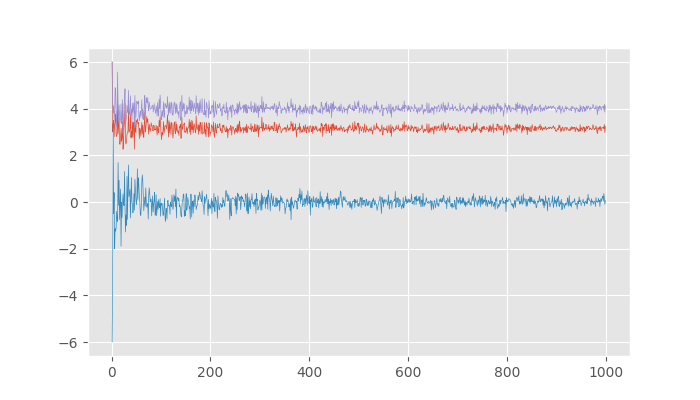
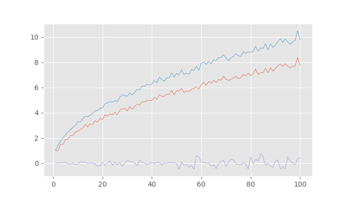
Looking at the distance traversed after taking a thousand iterations:

def steps(max_steps):
    distances = []
    rms_distances = []
    displacements = []
    steps = []
    
    for i in range(1, max_steps + 1):
        dist, rms, disp = all_stats(i, 1000)
        distances.append(dist)
        rms_distances.append(rms)
        displacements.append(disp)
        steps.append(i)

    plt.figure(figsize=(7,4))
    plt.plot(steps, distances, linewidth=.5)
    plt.plot(steps, rms_distances, linewidth=.5)
    plt.plot(steps, displacements, linewidth=.5)
    plt.savefig("../static/images/steps.png")

steps(100)

/tmp/babel-1rbHGK/python-6Z9dnp:14: RuntimeWarning: More than 20 figures have been opened. Figures created through the pyplot interface (`matplotlib.pyplot.figure`) are retained until explicitly closed and may consume too much memory. (To control this warning, see the rcParam `figure.max_open_warning`).
  plt.figure(figsize=(7,4))

It's fairly easy to derive the average root mean square distance after N steps:

• Represent a walk as the series of steps \(x_1\), \(x_2\), \(x_3\), … , \(x_n\). \(x_i\) can only be +1 or -1.
• The total distance at the end of the walk is \(x_1 + x_2 + x_3 + ... + x_n\).
• Let \(N\) be the total possible walks, which is \(2^n\) because at each of the \(n\) steps we have \(2\) options.
• Then, the square of the root mean square distance (just to allow simpler typing):

• \((x_{1,1}x_{2, 1} + x_{1,2}x_{2,2} + ...)\) evaluates to zero because it covers all possible combinations of pairs of values being added together: \(x_{i,k}x_{j,k}\) must be either \(1\) or \(-1\) depending on the individual values, with equal chance. Once we cover all possibilities, all the values cancel out.