A Simple Neural Network (<200loc, rust)
I've always enjoyed terse programs that show how things work without magic hiding incidental complexity. After realizing that my initial attempt at a neural net only cost less than 200 lines of Rust, I decided to take a snapshot and write about building it before I go on and extend (and possibly over-complicate or abandon) the system.
More than anything else, treat this as encouragement to write your own neural network – the core implementation turned out to be surprisingly compact – enough to encourage me to write about it.
This is not an introduction to neural nets: There are several excellent resources already available online that can describe the underlying math and structure of networks; I'll just talk through them enough to explain the structure of the code.
It's also entirely likely that I have mistakes in here; this was written quickly with the main aim of encouraging more people to write their own nets from scratch – and given one simple point for comparison. If you do write your own, please share it with me!
Choosing a simple problem & architecture
Achieving SotA on MNIST is an explicit non-goal: this project is aimed at exploring the mechanics of a neural network, and being able to play around with it while changing one feature at a time.
Instead of trying to see if the network can accurately predict results from data I can't understand or reason about, I'm going to have the network try to behave like a simple continuous function of my choice instead – I'll play with different functions like \(y=x^2\), \(y=x^3\), \(y=x * sin(x)\), etc.
This greatly simplifies some parts of the network – there's a single input, and single output. The Universality Theorem suggests that I should be able to get fairly far with a single layer, so that's where I'm starting.
I like ReLU and leaky ReLU because of their simplicity, and I'll stick with them here – though I don't have any strong justification about the choice of activation function yet.
Building the network
Storing a network
The very first decision was figuring out how to store the neural network – my very first attempt at doing this involved a lot of pure functions and state being passed around all over the place which quickly became messy – it was much more maintainable to have a single place to represent a neural network.
struct Net {
}
Happily enough, with the decision to have a single input and output, a single hidden layer means that there are only so many weights I need to store.
The overall structure is fairly simple:
    o
  /   \
x - o  - y
  .   .
   . .
    o
Before drawing in the calculations that need to happen, I'm going to introduce a system for indexing nodes which should make this much easier to talk about and parse:
          Layer ->
   +------------------------->
   |
N  |               0       1
e  |               |       |
u  |          0 -  o       .
r  |       /         \     .
o  | 0 - x -  1 -  o - 0 - y
n  |       .         .
|  |        .       .
v  |         ns -  o
   v
It's a fairly simple system for drawing neurons – a layer index that starts at the first hidden layer; and a per-layer index into the neuron itself.
For each weight in the system, there are going to be 3 coordinates: the neuron it's at, and then the input it's specified for – this is a little bit different than most online courses, because I'm not directly using vectors to be very explicit about the underlying calculations (both avoiding matrix calculations and paying the price in terms of speed as the price).
Drawing in the calculations for evaluating the network forward to make this a little bit more concrete:
         0    1
         |    |                   layer input
                                    |     |
     0 - o <------- n[0,0] = relu(w[0, 0, 0]x + b[0, 0, 0])
  /        \                           |
x -  1 - o -  y                      neuron
  .        .   \
   .      .     relu(sum(w[1, x, i]*n[0, i] + b[1, x, i]))
    ns - o
I also have somewhat stronger constraints on the potential values for my indexes:
- for layer = 0
- the neuron's index can go from 0 ->
ns(number of neurons) - the input can only be 0
- the neuron's index can go from 0 ->
- for layer = 1
- the neuron's index can only be 0 (just one output)
- and the input can go from 0 -> ns (# of neurons in previous layer)
In the code, I often refer to the [layer, neuron, input] index as [x,
y, z].
Having this written out explicitly helped me a lot in implementing the network, and I hope the constraints should make sense to you given the structure of the network.
Finally, instead of dealing with initializing and taking care of multi-dimensional vectors or arrays, I'm going to use a trick I often rely on in Advent of Code for complex grid structures and keep a single vector – with a function to translate my custom indexing system into offsets.
struct Net {
    ws: Vec<f64>,
    bs: Vec<f64>,
    ns: usize,
}

impl Net {

    pub fn new(ns: usize) -> Net {
        let size = ns * 2;
        let ws: Vec<f64> = vec![0; size]; // This will change
        let bs: Vec<f64> = vec![0; size];

        Net { ws, bs, ns }
    }

    pub fn pt(self: &Self, x: usize, y: usize, z: usize) -> usize {
        match x {
            0 if z == 0 && y < self.ns => y,
            1 if y == 0 && z < self.ns => self.ns + z,
            _ => panic!("Invalid location: {}, {}, {}", x, y, z),
        }
    }
}
Initializing the network
Starting the network with all weights initialized to 0 is a good way to get stuck with 0 gradients during gradient descent: and a good experiment to run while running the code yourself.
For this first iteration, I'm hard coding random initialization of weights into the program – but I'll expose another function that accepts custom initial weights in the next iteration for exploration.
+ use rand::thread_rng;
+ use rand::{distributions::Standard, Rng};

  impl Net {

      pub fn new(ns: usize) -> Net {
          let size = ns * 2;
-         let ws: Vec<f64> = vec![0; size]; // This will change
+         let ws: Vec<f64> = thread_rng().sample_iter(Standard).take(size).collect();
-         let bs: Vec<f64> = vec![0; size];
+         let bs: Vec<f64> = thread_rng().sample_iter(Standard).take(size).collect();

          Net { ws, bs, ns }
      }

  }
And a corresponding dependency in Cargo.toml:
[dependencies]
rand = "0.7.3"
I admit being disappointed about having to use an external crate that does have some magic, but RNGs are another black box to open and play with for another day.
Evaluating a single point
Up next is evaluating the value predicted by the network at a single point, which is a straight forward traversal through the network. I'm going to use a leaky ReLU as my activation function, so I'll quickly define it:
fn relu(v: f64) -> f64 {
    if v >= 0.0 {
        v
    } else {
        0.01 * v
    }
}
First, I'm going to throw in several utility functions to access or calculate values in different parts of the net – in my first implementation, I extracted these out after implementing back-prop, but there's no harm in putting them up here first.
impl Net {

    /// Relu(w * input + b) for coordinates x, y, z with input val
    fn rwxb(self: &Self, val: f64, x: usize, y: usize, z: usize) -> f64 {
        relu(self.wxb(val, x, y, z))
    }

    /// w * input + b for coordinates x, y, z with input val
    fn wxb(self: &Self, val: f64, x: usize, y: usize, z: usize) -> f64 {
        self.w(x, y, z) * val + self.b(x, y, z)
    }

    fn w(self: &Self, x: usize, y: usize, z: usize) -> f64 {
        self.ws[self.pt(x, y, z)]
    }

    fn b(self: &Self, x: usize, y: usize, z: usize) -> f64 {
        self.bs[self.pt(x, y, z)]
    }

}
Iterating through the net and calculating values lends itself comfortably to Rust's beautiful iterator/expression based system:
impl Net {
    pub fn eval(self: &Self, val: f64) -> f64 {
        relu(
            (0..self.ns)
                .map(|i| self.rwxb(self.rwxb(val, 0, i, 0), 1, 0, i))
                .sum(),
        )
    }
}
If you look at the diagram, I need to calculate the values of the
individual neurons – \(Relu(w * x + b)\) – which can be expressed as
rwxb(x, 0, i, 0) with x as the input and i ranging from 0 to ns
(number of neurons).
Then, the value of y is the value of these neurons as inputs added up, and passed through Relu again. Which is exactly what the function above does.
(I admit to messing up the naming convention a little bit with x playing double duty as both the input and the first coordinate; I'll try to clean this up later if I find anyone actually reading this post.)
Expenses
Keeping loss as simple as possible, I'm simply calculating it as \((y - y')^2\) at a data point. The cost, or loss across a given set of data is then the average of the total loss. The implementation is as straightforward as you would expect, given data in the form of tuples.
This is yet another decision to play around with in the future with alternative functions.
impl Net {
    pub fn cost(self: &Self, data: &[(f64, f64)]) -> f64 {
        let mut loss = 0.0;
        for (x, y) in data {
            let val = self.eval(*x);
            loss += (y - val).powi(2);
        }
        loss / self.ns as f64
    }
}
Training!
Training involves calculating the cost for a given set of inputs, determining the gradients of the cost for that set of inputs in terms of all the weights and biases.
And then updating the weights and biases with the given learning rate – which involves even more decisions and hyperparameters.
Determining the gradient
This was the hardest part of the whole exercise: packages like Pytorch
allow automating the gradient calculation – by swapping out the
implementation of all the other mathematical functions, and
transparently converting that to the gradient with autodiff.
Instead of building a system to do automatic differentiation, I
decided to do things by hand for my simple function. I'll start off
with getting some utility functions out of the way to start – the
differential of Relu depends on the value of the original function, so
I extracted relu_ish out of the implementation.
/// Leaky relu
fn relu(v: f64) -> f64 {
    relu_ish(v, v)
}

/// Leaky relu based on another variable, useful for derivatives
fn relu_ish(v: f64, point: f64) -> f64 {
    if point >= 0.0 {
        v
    } else {
        0.01 * v
    }
}
Some rough calculations for the basis of the next function:
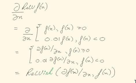
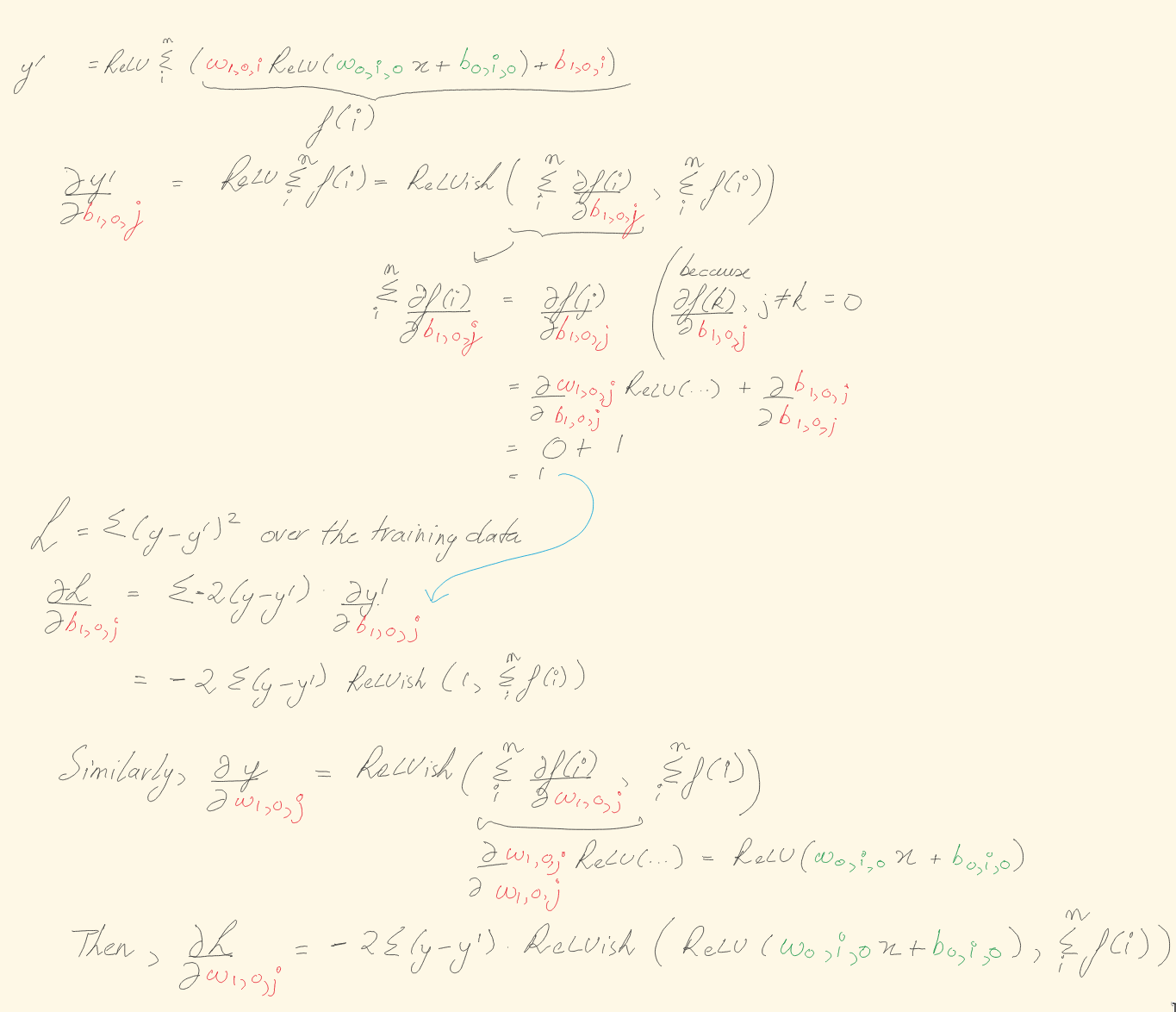
Figure 1: Calculating some of the gradients
The source code below is after some clean up – after directly writing out the calculations, I simply extracted and re-used some common variables and loops.
The adjustments to be made are first calculated and then applied, to prevent the order of evaluation affecting the rest of the calculation.
impl Net {
  fn backprop(self: &mut Self, data: &[(f64, f64)], learning_rate: f64) {
      let mut dws: Vec<f64> = vec![0.0; self.ns * 2];
      let mut dbs: Vec<f64> = vec![0.0; self.ns * 2];

      for i in 0..self.ns {
          let pt1 = self.pt(0, i, 0);
          let pt2 = self.pt(1, 0, i);

          for (x, y) in data {
              let yy = self.eval(*x);

              dws[pt2] += -2.0 * (y - yy) * relu_ish(self.rwxb(*x, 0, i, 0), yy);
              dbs[pt2] += -2.0 * (y - yy) * relu_ish(1.0, yy);

              dws[pt1] += -2.0 * (y - yy) * relu_ish(self.ws[pt2] * relu_ish(*x, self.wxb(*x, 0, i, 0)), yy);
              dbs[pt1] += -2.0 * (y - yy) * relu_ish(self.ws[pt2] * relu_ish(1.0, self.wxb(*x, 0, i, 0)), yy);
          }
      }

      for i in 0..self.ns {
          for pt in &[self.pt(1, 0, i), self.pt(0, i, 0)] {
              self.ws[*pt] -= dws[*pt] * learning_rate;
              self.bs[*pt] -= dbs[*pt] * learning_rate;
          }
      }
  }
}
Finally, training is pretty simple: break the input data into pieces to train each batch, and loop through it all. I like to record the total cost at a reasonable interval – to get a total of 10 data points around how cost is proceeding to give me a sense of the nets behavior.
impl Net {
    pub fn train(
        self: &mut Self,
        training_data: &[(f64, f64)],
        epochs: usize,
        batch_size: usize,
        learning_rate: f64,
    ) {
        let log_interval = epochs / 10;

        for epoch in 0..epochs {
            let mut point = 0;
            while point <= training_data.len() {
                let limit = min(point + batch_size, training_data.len());
                self.backprop(&training_data[point..limit], learning_rate);
                point += batch_size;
            }

            if log_interval > 0 && epoch % log_interval == 0 {
                eprintln!("Epoch {}: {}", epoch, self.cost(training_data));
            }
        }
    }
}
Training the net to a function
The actual training is fairly anticlimatic: I use a lambda to generate training and validation data, and then print out what I see. Tweaking the hyperparameters has been extremely fascinating; my obvious next step from here on is to run the net multiple times and demonstrate the differences in behavior by changing the hyperparameters.
To be able to quickly visualize the results, I also printed out a 1000 data points for gnuplot.
fn main() {
    fn original_fn(x: f64) -> f64 {
        x * x * x + x * x + x
    };

    let training_data: Vec<(f64, f64)> = (1..=100)
        .step_by(7)
        .map(|x| (x as f64) / 100.0)
        .map(|x| (x, original_fn(x)))
        .collect();

    let validation_data: Vec<(f64, f64)> = (20..=60)
        .map(|x| (x as f64) / 100.0)
        .map(|x| (x, original_fn(x)))
        .collect();

    let start = Instant::now();
    let mut net = Net::new(20);
    net.train(&training_data, 100000, 100, 0.000001);
    eprintln!("Training duration: {}s", start.elapsed().as_secs());
    eprintln!("Validation error: {}", net.cost(&validation_data));

    for x in 0..1000 {
        let x = x as f64 / 1000.0;
        println!("{}\t{}\t{}", x, original_fn(x), net.eval(x));
    }
}
Running this with (using release took my training time from ~147s to 7s!)
cargo run --release > x3
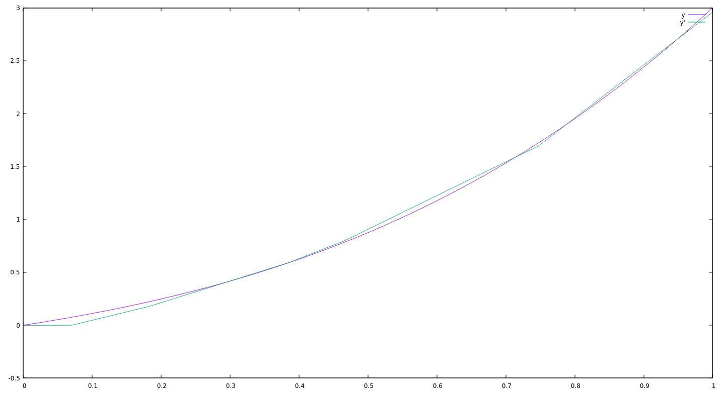
and plotting in gnuplot with
gnuplot> plot "x3" using 1:2 title "y" with lines, "x3" using 1:3 title "y'" with lines
Results in a fairly satisfying graph:
What's next?
The very first step is going to be unit-tests: I found a bug in how I was doing back-propagation right before publishing this post. I've learned this lesson so many times but it clearly hasn't sunk in enough – data science and ML can be extremely deceiving – and it's far too easy to get a result that looks correct, but isn't.
With this skeleton in place, I'm going to be playing with extending this to support multiple layers – which means a slightly more simplified implementation for differentiation that, and then implement searching through hyperparameters to find the "best" results automatically – and show me the search space at the same time.
And of course, I also plan to keep iterating on this for speed – including profiling and adding true vectors, adding behaviors like regularization, etc. to explore how things work and how the weights changed. I have to admit I'm fairly excited to have code that I can very comfortably tweak under extremely controlled conditions, making it possible for me to iterate quickly and learn fast.
The full source code
//! A naive neural network implementation
//! with all fully connected layers

//! Starting with a single layer net,
//! with one input and one output
//! ```
//!          0    1
//!          .    .
//!          .    .          neuron position
//!                               -v--v-
//!      0.. o <- n[0,0] = relu(w[0, 0, 0]x + b[0, 0, 0])
//!    /       \                        -^- input position
//! x -- 1.. o -- y <- relu(sum(w[1, x, i]*n[0,i] + b[1, x, i]))
//!    \       /
//!      2.. o
//!
//!
//! ```

use rand::thread_rng;
use rand::{distributions::Standard, Rng};
use std::cmp::min;
use std::time::Instant;

/// Data structure to hold the net
struct Net {
    ws: Vec<f64>,
    bs: Vec<f64>,
    ns: usize,
}

impl Net {
    /// Create a fully-connected net with hidden layer size
    pub fn new(ns: usize) -> Net {
        let size = ns * 2;
        let ws: Vec<f64> = thread_rng().sample_iter(Standard).take(size).collect();
        let bs: Vec<f64> = thread_rng().sample_iter(Standard).take(size).collect();

        Net { ws, bs, ns }
    }

    /// Calculates an index into the weights/biases vector
    /// for a given net
    pub fn pt(self: &Self, x: usize, y: usize, z: usize) -> usize {
        match x {
            0 if z == 0 && y < self.ns => y,
            1 if y == 0 && z < self.ns => self.ns + z,
            _ => panic!("Invalid location: {}, {}, {}", x, y, z),
        }
    }

    pub fn train(
        self: &mut Self,
        training_data: &[(f64, f64)],
        epochs: usize,
        batch_size: usize,
        learning_rate: f64,
    ) {
        let log_interval = epochs / 10;

        for epoch in 0..epochs {
            let mut point = 0;
            while point <= training_data.len() {
                let limit = min(point + batch_size, training_data.len());
                self.backprop(&training_data[point..limit], learning_rate);
                point += batch_size;
            }

            if log_interval > 0 && epoch % log_interval == 0 {
                eprintln!("Epoch {}: {}", epoch, self.cost(training_data));
            }
        }
    }

    pub fn cost(self: &Self, data: &[(f64, f64)]) -> f64 {
        let mut loss = 0.0;
        for (x, y) in data {
            let val = self.eval(*x);
            loss += (y - val).powi(2);
        }
        loss / self.ns as f64
    }

    fn backprop(self: &mut Self, data: &[(f64, f64)], learning_rate: f64) {
        let mut dws: Vec<f64> = vec![0.0; self.ns * 2];
        let mut dbs: Vec<f64> = vec![0.0; self.ns * 2];

        for i in 0..self.ns {
            let pt1 = self.pt(0, i, 0);
            let pt2 = self.pt(1, 0, i);

            for (x, y) in data {
                let yy = self.eval(*x);

                dws[pt2] += -2.0 * (y - yy) * relu_ish(self.rwxb(*x, 0, i, 0), yy);
                dbs[pt2] += -2.0 * (y - yy) * relu_ish(1.0, yy);

                dws[pt1] += -2.0 * (y - yy) * relu_ish(self.ws[pt2] * relu_ish(*x, self.wxb(*x, 0, i, 0)), yy);
                dbs[pt1] += -2.0 * (y - yy) * relu_ish(self.ws[pt2] * relu_ish(1.0, self.wxb(*x, 0, i, 0)), yy);
            }
        }

        for i in 0..self.ns {
            for pt in &[self.pt(1, 0, i), self.pt(0, i, 0)] {
                self.ws[*pt] -= dws[*pt] * learning_rate;
                self.bs[*pt] -= dbs[*pt] * learning_rate;
            }
        }
    }

    pub fn eval(self: &Self, val: f64) -> f64 {
        relu(
            (0..self.ns)
                .map(|i| self.rwxb(self.rwxb(val, 0, i, 0), 1, 0, i))
                .sum(),
        )
    }

    /// Relu(wx + b) for coordinates x, y, z with input val
    fn rwxb(self: &Self, val: f64, x: usize, y: usize, z: usize) -> f64 {
        relu(self.wxb(val, x, y, z))
    }

    /// wx + b for coordinates x, y, z with input val
    fn wxb(self: &Self, val: f64, x: usize, y: usize, z: usize) -> f64 {
        self.w(x, y, z) * val + self.b(x, y, z)
    }

    fn w(self: &Self, x: usize, y: usize, z: usize) -> f64 {
        self.ws[self.pt(x, y, z)]
    }

    fn b(self: &Self, x: usize, y: usize, z: usize) -> f64 {
        self.bs[self.pt(x, y, z)]
    }
}

/// Leaky relu
fn relu(v: f64) -> f64 {
    relu_ish(v, v)
}

/// Leaky relu based on another variable, useful for derivatives
fn relu_ish(v: f64, point: f64) -> f64 {
    if point >= 0.0 {
        v
    } else {
        0.01 * v
    }
}

fn main() {
    fn original_fn(x: f64) -> f64 {
        x * x * x + x * x + x
    };

    let training_data: Vec<(f64, f64)> = (1..=100)
        .step_by(7)
        .map(|x| (x as f64) / 100.0)
        .map(|x| (x, original_fn(x)))
        .collect();

    let validation_data: Vec<(f64, f64)> = (20..=60)
        .map(|x| (x as f64) / 100.0)
        .map(|x| (x, original_fn(x)))
        .collect();

    let start = Instant::now();
    let mut net = Net::new(20);
    net.train(&training_data, 100000, 100, 0.000001);
    eprintln!("Training duration: {}s", start.elapsed().as_secs());
    eprintln!("Validation error: {}", net.cost(&validation_data));

    for x in 0..1000 {
        let x = x as f64 / 1000.0;
        println!("{}\t{}\t{}", x, original_fn(x), net.eval(x));
    }
}
[package]
name = "nn"
version = "0.1.0"
authors = ["Kunal Bhalla <bhalla.kunal@gmail.com>"]
edition = "2018"

[dependencies]
rand = "0.7.3"
Comments? Feedback? Suggestions?
Drop me an email or reach out on Twitter @kunalbhalla.
History
- 2020-11-29: Published first version.